Uncategorized

W. Edwards Deming’s Contributions to the Practice of Analytics

May 10, 2021 by Robert Grossman

In this post, we continue our profiles of individuals who have made contributions to the practice of analytics by discussing the life and work of W. Edwards Deming. As I will explain below, it may be helpful to think of statistical quality control in the 1950’s and 1960’s as playing some of the same role that predictive analytics did in the last decade and that AI does in this decade.

Deming made a number of contributions to the practice of analytics, but in my opinion, three of the most important were:

Developing and refining a process loop (Deming Cycle) for improving quality.
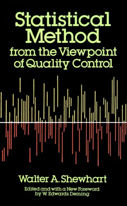
Organizing Walter Shewhart’s notes about statistical process control and editing them to produce an influential book that was published in 1939. The book is still available as a Dover reprint for less than $15 and still worth reading.
Bridging sampling methodology with the practical practice of statistical quality control and teaching thousands of people about it in seminars, tutorials, and consulting engagements, including in a series of influential seminars in Japan after World War II.

Why does Deming and his influence on statistical process control in the 40’s – 80’s matter today? The reason is simple. We have good software frameworks for building analytic models and many textbooks about deep learning, but little practical advice about how to build high quality systems with embedded deep learning. To say it simply, we could use some Demings for deep learning.

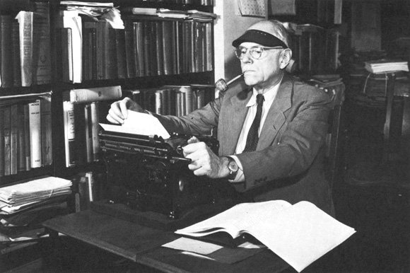
In this post, I’ll cover four facts about Deming that provide a perspective on his importance on the practice of analytics. From the viewpoint of the analytic diamond, Deming had a deep knowledge and important insights both about analytic modeling (the technical foundations and methodology) and analytic operations (part of the practice of analytics). But this is not the reason that most people in analytics know his name today. First, he was in the right place at the right time –with the US government during the World War II where quality was critical for the industrial productivity required to beat the Axes powers and in Japan during its postwar reconstruction where quality was critical for pivoting Japanese industry towards high quality manufacturing. Second, his emergence as a guru was catalyzed by a 1980 NBC documentary about him. Prior to the documentary, he was relatively unknown.

Understanding the contributions of W. Edwards Deming to the practice of analytics is not as simple as it as first appears. The British Library has a nice balanced assessment [1]:

"William Edwards Deming (1900-1993) is widely acknowledged as the leading management thinker in the field of quality. He was a statistician and business consultant whose methods helped hasten Japan’s recovery after the Second World War and beyond. He derived the first philosophy and method that allowed individuals and organisations to plan and continually improve themselves, their relationships, processes, products and services."
Source: W. Edwards Deming, https://www.bl.uk/people/w-edwards-deming.

Deming’s Early Career and Two Defining Events

Deming (1900-1993) received a M.S. from the University of Colorado, Boulder in 1924 in mathematics and mathematical physics and a PhD from Yale University in 1928 in mathematical physics [7].

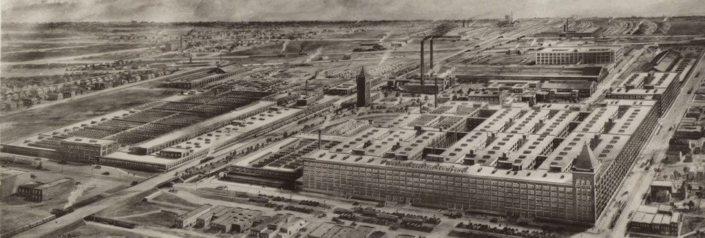
The first defining event in Deming’s education was the time he spent over the summers of 1925 and 1926 as an hourly worker at Western Electric’s Hawthorne Works in Cicero, near Chicago [7]. Telephone equipment was mass produced at Hawthorne Works, which employed over 45,000 workers in factory conditions that were extremely monotonous. Deming’s time at the Hawthorne Works gave him first hand knowledge about assembly lines and the complex interaction of mechanical processes, human processes, and the different types of variations that resulted.

Hawthorne Works was the home for several critical studies in industrial management. During 1924-1932, what became known as the Hawthorne Experiments on industrial productivity were conducted there. Although, Deming was not directly involved in them, one of the results of the Hawthorne Experiments and similar work was the emergence of the human relations movement within management studies that balanced Frederick Taylor’s scientific management movement. (Note that the Hawthorne Experiments were related to, but different, then what later became known as the Hawthorne Effect [9].)

The Western Electric Hawthorne Works factory complex in Cicero, Illinois in 1925.

In 1927, Deming took a job at the US Department of Agriculture (USDA). While there, he was introduced to Walter A. Shewhart of the Bell Telephone Laboratories. The second defining event of his early career is that Deming edited a series of lectures delivered by Shewhart at USDA. This became the book by Shewhart called Statistical Method from the Viewpoint of Quality Control that was published in 1939 [6]. The material covered in the lectures included the core concepts of statistical quality control and the control chart.

The book Statistical Method from the Viewpoint of Quality Control by Walter A. Shewhart that was published in 1939 and reprinted in 1986. The book was edited by Deming.

Deming’s Technical Mastery of the Statistical Process Control

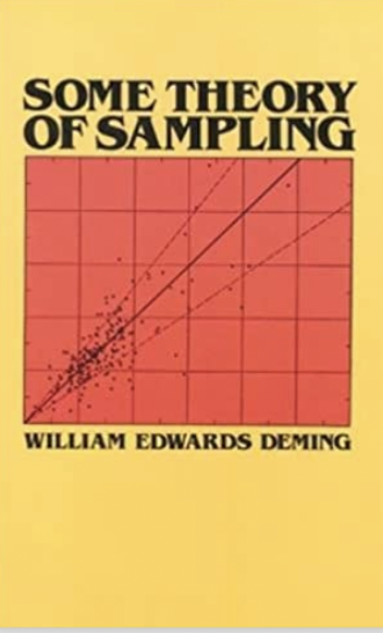
Fact 1. Deming had a deep technical understanding of the field of statistical process control. Deming understood all the mathematics and statistical required and spent over two decades practicing statistical process control. He collected and organized this technical material into a 602 page book called Some Theory of Sampling that was published by John Wiley & Sons in 1950 [2]. The book was reviewed in 1951 in the Journal of the American Statistical Association:

The information in this book is so extensive that the presentation may appear bewildering at first glance. But once the reader gets acquainted with its contents, it becomes clear that the topics are developed logically and systematically. It seems likely that for some time to come this book will be the "bible" of sampling statisticians [4].

The information in this book is so extensive that the presentation may appear bewildering at first glance. But once the reader gets acquainted with its contents, it becomes clear that the topics are developed logically and systematically. It seems likely that for some time to come this book will be the “bible” of sampling statisticians.

W. Edwards Deming book Some Theory of Sampling was published in 1950.

Deming as a Practitioner

Fact 2. Deming was a great practitioner of statistical quality control. Deming gained over a decade of practical experience at the Department of Agriculture, Census Bureau and Department of Defense with statistical process control before he advised the Japanese manufacturing community during the reconstruction after World War II.

Deming as a Teacher – The Red Beads Experiment

Fact 3. Deming was a great teacher.

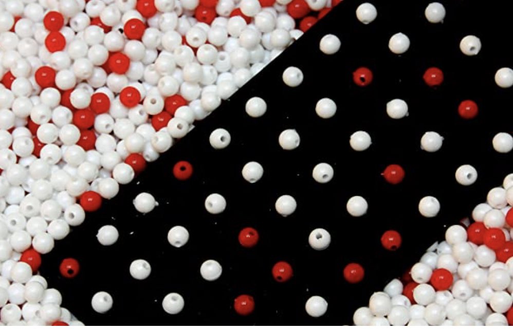
The Red Beads Experiment was a three day experiment that Deming used as the core in many of his tutorial introductions to statistical process control. The description here follows [5]. Deming began using the red bead experiment in the early 1980’s.

The Red Bead Experiment uses a control chart (also known as a process behavior chart) to show that even though a 'willing worker' wants to do a good job, their success is directly tied to and limited by the nature of the system they are working within. Real and sustainable improvement on the part of the willing worker is achieved only when management is able to improve the system, starting small and then expanding the scope of the improvement efforts.
Source: Red Bead Experiment, accessed from: https://deming.org/explore/red-bead-experiment/

The red bead experiment uses the following:

box of wooden beads, with 3,200 white beads and 800 red beads
a paddle with with fifty bead size holds
a box for mixing the beads
six workers
two inspectors who count the beads produced using the paddles
a chief inspector who verifies the counts
an accountant who records the counts
and a customer who accepts only white beads

The goal is for each worker to produce fifty white beads per day. The process starts by mixing the beads using the two boxes. Next each of the six workers dips the paddle into the larger box without shaking it, carries the paddle to each inspector for counting and verification, and then dumps the paddle back into the larger box, so the next worker can repeat the process.

After each of the six workers completes this process (thought of as corresponding to one day), the manager makes decisions about how best to reward the successful workers (those that produced the most white beads) and how to put in place performance improvement plans for the least successful workers (those whose work had the most red beads). Of course, who produces the most white beads and the most red beads is a random process, and nothing can change until the production line / process itself changes.

By carrying out the process for four rounds (corresponding to days) and analyzing the experiment over days of instruction provided an opportunity for thoroughly covering everything from the sampling approach and how to manage, to the variation between workers, and how what appeared to be differences in the talent of the scoopers was nothing more than normal variation.

Deming used 4 paddles over the 45 years that he used the red bed experiment in his teaching and kept track of the mean number of red beads for each paddle. It was 11.3, 9.6, 9.2 and 9.4 [3].

Those that took Deming’s three day course learned a lot from them. These days, when instruction is so different, it might be hard to understand this, but Deming intermixed sampling theory from binomial distributions, with understanding natural variation, with understanding how to manage and reward workers, with advice how to diagnose and improve industrial systems and processes. In our language, it intermixed both analytics models/analytic methodologies with the practice / management of analytics, something that is rare today, despite the number of data science boot camps.

The red bead experiment uses 3200 white beads, 800 red bead, and a collecting paddle with 5 x 10 holes, each of which can hold one bead. The goal is to collect 50 white beads.

The Role of the NBC Documentary “If Japan Can, Why Can’t We?”

Fact 4. Deming was in the right place at the right time, and the 1980 NBC documentary was a catalyst. A critical role was played by the 1980 NBC documentary “If Japan Can, Why Can’t We?” A very thoughtful discussion of the importance of this documentary is provided in the analysis by William M. Tsutsui in [8].

Immediately after the documentary, CEOs from US companies wanted Deming to teach their workers how to improve quality, and his fame grew substantially [8].

References

[1] British Library, W. Edwards Deming, https://www.bl.uk/people/w-edwards-deming, accessed on May 10, 2021.

[2] Deming, W. Edwards, Some Theory of Sampling, John Wiley & Sons, 1950. Reprinted Dover Publications, 1984.

[3] Deming, W. Edwards. 1993. The New Economics for Industry For Industry, Government & Education. MA. Massachusetts Institute of Technology Center for Advanced Engineering Study. Chapter 7.

[4] Frankel, Lester R. Journal of the American Statistical Association 46, no. 253 (1951): 127-29.

[5] Martin, James R., What is the Red Bead Experiment, https://maaw.info/DemingsRedbeads.htm, accessed on May 12, 2021.

[6] Shewart, Walter, Statistical Method from the Viewpoint of Quality Control, US Department of Agriculture, 1939.

[7] The W. Edwards Deming Institute, Timeline, accessed from https://deming.org/timeline/ on May 2, 2021.

[8] Tsutsui, W.M., 1996. W. Edwards Deming and the origins of quality control in Japan. Journal of Japanese Studies, 22(2), pp.295-325.

[9] Wickström, G. and Bendix, T., 2000. The “Hawthorne effect”—what did the original Hawthorne studies actually show?. Scandinavian journal of work, environment & health, pages 363-367.

Lessons from the Ever Given and Archegos: Four Ways Predictive Models Fail

April 9, 2021 by Robert Grossman

The Hierarchy of Uncertainty and Why Models Break Down

Figure 1. The container ship Ever Given blocking the Suez Canal (2021). Source: Copernicus Sentinel data (2021), processed by Pierre Markuse.

In the news over the past month was the story of how the Ever Given blocked the Suez Canal and stopped an estimated 10% of global shipping and how the collapse of Archegos Capital Management led to billions of dollars of losses, including $2 billion of losses for Nomura, Japan’s largest bank, and $5 billion of losses from Credit Suisse, an investment banking company headquartered in Switzerland. Lloyd’s of London is expected to have losses of approximately $100 million from the delay to shipping that it insured.

Banks run multiple types of risk models to protect themselves from these types of events from happening, as do insurance companies. In this post, we examine some of the reasons that predictive models have trouble with these types of losses and what can be done about it. More generally, we look at the types of uncertainty that arise when building machine learning and AI models.

The Hierarchy of Unknowns in Machine learning

We assume that we have a predictive risk model that has inputs or features. It is quite helpful to distinguish between four types of unknowns and to view these as forming a hierarchy.

Known stochastic variance. Stochastic here simply means that the inputs or features are not deterministic but instead vary and that the variances can be described by a probability distributions. This is the normal state of affairs for most models. These types of models have false positives and false negatives, but are the types of models that data scientists build routinely. One of the ways that these types of models can break down is through drift – over time the behavior that models attempt to capture tends to drift and models might be updated and re-estimated to capture this drift.
Unknown stochastic variance. It’s common not to have enough data to be able to characterize the probability distributions of the variables driving your model. In this case, getting more data is critical. A particular challenge are long tailed distributions, or distributions associated with power laws, since this can create situations in which collecting enough data is particularly challenging. There are a number of specialized techniques used in this case, such as catastrophe modeling (“cat modeling“), which is used to predict catastrophic losses, such as losses associated with earthquakes or hurricanes.
Unknown variables, features, actors and interactions. In practice, models are approximate and usually do not have all the relevant features. Overtime, as modelers understanding improves, additional features can be added to improve the performance of the model. These days this is often done by using large amounts of data and using deep learning to create features automatically. This is a very effective approach, but the larger the data, the more likely it is to be biased, which introduces biases into the model.
New behavior, new interactions and actors. As container grew in size, they became large enough to block the canal, a new behavior. You can also think of this as an emergent behavior, since the size of ships has been increasing for a long time, but as the size increases past certain thresholds new types of behavior emerge, such as blocking a particular canal. As another example, one of the reasons that Archegos Capital collapse is the instability caused by a new type of complex financial instrument called a total return swap [2], which again you can think of a new type of behavior associated with a new type of financial instrument.

The Difference Between Level 2 and Level 3 Uncertainty

It’s standard in data science to distinguish between risk and uncertainty: You are dealing with risk when you know all the alternatives, outcomes and their probabilities (Level 1 uncertainty above). You are dealing with uncertainty when you do not know all the alternatives, outcomes or their probabilities (Level 2 or higher levels of uncertainty above).

The Difference Between Level 3 and Level 4 Uncertainty

There is a subtle but critical difference between Level 3 and Level 4 uncertainty. With Level 3 uncertainty, the features, actors, or interactions are present, but not yet understood and not yet included in the model. Once identified, there may, or may not, be enough data to accurately model their distribution (the difference between Level 1 and Level 2 variables and features). With Level 4 Uncertainty, new behavior appears, such as the use by investors of total return swaps, or the transportation of containers by ships so large that they can completely block a canal.

Black Swans

A black swan can be defined as an unpredictable or unforeseen event, typically one with extreme consequences. Black swan events were popularized by Nassim Talab in his influential book by that name [3]. The term “black swan” has been used since the second century to refer to something impossible or unlikely, since only white swans were seen by Europeans until a black swan was seen by Dutch explorers visiting Australia in 1697.

Black swans can arise from the behaviors 2, 3 and 4 in the hierarchy of uncertainty. For example, they can arise when tail events occur in Level 2 uncertainty, when behavior that is not yet identified occurs in Level 3 uncertainty, or when new behavior or actors arise in Level 4 uncertainty.

Talab has importantly pointed out the fragile and unstable state that often occurs due to new interactions that arise, such as the excessive risk taking by banks, the bursting of the housing bubble, and credit illiquidity that led to the 2007-2008 financial crisis [4].

Deep Uncertainty

Another way of thinking of the different types of uncertainty in the hierarchy of uncertainty is through the concept of deep uncertainty. One definition of deep uncertainty is [5]:

Likelihood of future events & outcomes cannot be well-characterized with existing data and models
Uncertainty cannot be reduced by gathering additional information
Stakeholders disagree on consequences of actions

There is an emerging field called modeling under deep uncertainty (MUDU) which is establishing best practices for building models with deep uncertainty [5].

Best Practices

Figure 2 summarizes some best practices when faced with different types of uncertainty. With Level 1 uncertainty, simply improving the model helps, while re-estimating the model is necessary to manage drift. With Level 2 uncertainty, getting more data can help. It’s critical to understand whether the variable is long tailed and whether a power law is involved. If so, it may not be likely that you will get enough data before a black swan like event occurs. With Level 3 uncertainty, it’s more about gaining more insight into root causes, external interactions, the robustness of the system than improving the model. Finally, with Level 4 uncertainty, the best approach is to develop more caution and try to be quicker to detect new actors and new interactions and to take appropriate actions than your competitors.

References

[1] Container Ship ‘Ever Given’ stuck in the Suez Canal, Egypt – March 24th, 2021. Contains modified Copernicus Sentinel data [2021], processed by Pierre Markuse (License: Creative Commons Attribution 2.0 Generic)

[2] Quentin Webb, Alexander Osipovich and Peter Santilli, Wall Street Journal, March 30, 2021, What Is a Total Return Swap and How Did Archegos Capital Use It?

[3] Taleb, Nassim Nicholas. The black swan: The impact of the highly improbable. Vol. 2. Random house, 2007.

[4] Taleb, Nassim Nicholas. Antifragile: Things that gain from disorder. Vol. 3. Random House Incorporated, 2012.

[4] Walker, Warren E., Robert J. Lempert, and Jan H. Kwakkel. “Deep uncertainty.” Delft University of Technology 1, no. 2 (2012).

Profiles in Analytics: Frank Knight

March 15, 2021 by Robert Grossman

Frank Knight at work. Source: University of Chicago Library, https://www.lib.uchicago.edu/media/images/Knight.original.jpg.

I have written several short profiles in this blog about individuals that have contributed to the practice of analytics or made intellectual contributions that can be applied to the practice of analytics, including:

Claude Hopkins: An Early Advocate of Test Measure and Refine
George Heilmeier: Twelve Rules for a Chief Analytics Officer, which covers Heilmeier’s Catechism and Heilmeier’s Twelve Rules for a new CIO and adapts them to the duties of a Chief Analytics Officer
William H. Foege: Why Great Machine Learning Models are Never Enough: Three Lessons About Data Science from Dr. Foege’s Letter
In Chapter 8 of my book Developing an AI Strategy: a Primer, I also provide brief profiles of Kenneth R. Andrews (1916-2005) and his four step process for strategic planning; H. Igor Ansoff (1918–2002) and what is now called the Ansoff Matrix; and, Bruce D. Henderson (1915-1992) and the experience curve.

In this post, I want to discuss some of Frank Knight’s insights about risk [1] and how they can be applied to the practice of analytics today.

Frank Knight and the Chicago School of Economics

Frank Knight (1885 – 1972) was a professor of economics at the University of Chicago from 1928 to 1955, where he was one of the founders of what became known as the Chicago School of Economics. His students included three Nobel prize winners in economics: Milton Friedman, George Stigler and James M. Buchanan.

His intellectual interests were broad and stretched from economics to social policy, political history and philosophy. He taught courses in the history of economic thought, the relationship between economics and social policy, and was one of the founding faculty members of the University’s of Chicago Committee on Social Thought in the early 1940s [2]. He was (cross)-appointed as a Professor of Social Science in 1942, a Professor of Philosophy in 1945, and was named the Morton D. Hull Distinguished Service Professor in 1946 [2].

Frank Knight’s Book – Risk, Uncertainty and Profits

In this post, I would like to discuss the important distinction between risk and uncertainty that Knight introduced in his 1921 book Risk, Uncertainty and Profit [1], which was based on his PhD dissertation. (The book is now in the public domain.) One of his key insights was that perfect competition would not eliminate profits, since even with perfect competition different firms would make different judgements due to the presence of uncertainty, which he distinguished from risk.

Modeling risk vs planning for uncertainty. At the most basic level, phrased as we would describe it today, Knight distinguished risk and uncertainty this way: you are modeling risk, when you know the different variables, alternatives and outcomes and can estimate their probabilities. You are planning for uncertainty, when you do not know or cannot measure the relevant variables, alternatives and outcomes and are developing plans and mechanisms to deal with this uncertainty.

It is interesting to note that when Knight’s book was published in 1921, mathematics and econometric modeling had not yet dominated the field and his entire book (at least from a quick scan) does not contain a single equation, although I counted six graphs illustrating concepts such as supply and demand.

Modeling Risk vs Planning for Uncertainty

When modeling risk, you can use standard machine learning models. When planning for uncertainty, you need to consider different scenarios and try to create appropriate plans for those you can imagine and even those that are challenging to image. As an example, planning for uncertainty includes thinking about what today we we would call black swan events [3].

Another way to look at this distinction, is that risk is about objective probabilities about events that can be measured, while uncertainty is about subjective probabilities about events that have to be postulated. Both are important in the practice of analytics.

A third way to look at this distinction was described in his book using markets. If there is a market so that you can insure against some unknown outcome, it is risk; if there is not a market, it is uncertainty [1].

Knight viewed entrepreneurs as those willing to put with uncertainty in certain circumstances and and to manage it in search of profits [1].

As more and more complicated risk instruments were developed over the years, fewer outcomes could be classified as uncertainty. On the other, as more and more complicated risk instruments were introduced, uncertainty increased, fragility increased, and the number of unknown unknowns increased. This created situations in which markets could collapse, such as the 2008 financial collapse, with mortgage backed securities introducing their set of uncertainties.

Risk, Uncertainty and the Practice of Analytics

In last month’s post, I discussed the importance of distinguish between developing analytic models, developing a system that employs analytics, and growing an analytics business. Recall that I use the term analytics to include machine learning, data science, statistical modeling, and AI. Let’s apply Knight’s distinction between risk and uncertainty to analytics models, systems, and businesses.

Quantifying risk when developing models. I have found it helpful at times to apply Knight’s insight about the distinction between risk and certainty to the practice of analytics. When developing machine learning or AI models, it’s important to quantify the errors and risks associated with a model by understanding the stochastic nature its inputs, hidden variables, and outputs and being able to describe their probability distributions. It’s equally important to be able to estimate the confidence level of the parameters in the model.

Managing uncertainty when developing ML or AI systems. On the other hand when developing systems that use machine learning (ML) or AI, it’s important to use engineering best practices to reduce the impact of uncertainty. For example, a best practice is “fuzz the system” that you are building by sending noise as inputs for days on end to make sure that the system performs gracefully no matter what inputs are provided, even non-numeric inputs, not printing characters, etc. Although fuzzing is standard in testing software for security vulnerabilities, it is also an excellent method to test AI-based systems to make sure they perform well in practice. Another standard best practice is to exponentially dampen temporally varying input variables in a system so that the system provides approximately good predictions even when one or two temporally varying inputs are in error.

Managing uncertainty in ML or AI businesses. Finally, uncertainty is also critical in building profitable machine learning or AI businesses. Good business strategies are robust in the sense they survive not just contingencies that are likely and predictable, but also those in which there is not enough data to quantify the risk and those that involve outcomes that have not yet been observed. Today, we might talk about how a business can survive disruptive changes in a market, but this can also be thought of a type of what is sometimes called Knightian uncertainty.

References

[1] Knight, Frank Hyneman. Risk, uncertainty and profit. Houghton Mifflin, 1921. The book is in the public domain and a copy can be found here.

[2] University of Chicago Library, Guide to the Frank Hyneman Knight Papers 1908-1979, University of Chicago Frank Hyneman Knight Special Collection.

[3] Taleb, Nassim Nicholas. The black swan: The impact of the highly improbable. Random house, 2007.

How to Navigate the Challenging Journey from an AI Algorithm to an AI Product

February 15, 2021 by Robert Grossman

Figure 1. The journey from an AI algorithm or model to an AI system, an AI product and finally an AI business.

From an AI Algorithm to a FAIR and Robust AI Algorithm

It’s a long challenging journey from an AI algorithm to an AI product. These days there is a lot of focus on removing the bias of many AI algorithms, which is absolutely critical, but just one of the many things that must be done to go from an AI algorithm to an AI product.

Biased Algorithms

I spent over a decade building and deploying machine learning predictive models in regulated industries, such as financial services and insurance, and the assumption was that your models tended to be biased and you worked hard not only to identity and remove any biases, but also in preparing a case to regulators showing that your models were fair. Today, with all the advances in AI, we are in a different place. We have plenty of data and machine learning frameworks that make it much easier to build models. We now build models over large, obviously biased datasets, don’t take the time to look for biases, and then act surprised when third parties examine our models and find biases.

This reminds me a bit of the gambling scene in the film Casablanca:

Rick: How can you close me up? On what grounds?
Captain Renault: I’m shocked, shocked to find that gambling is going on in here!
[a croupier hands Renault a pile of money]
Croupier: Your winnings, sir.
Captain Renault: [sotto voce] Oh, thank you very much.
Captain Renault: [aloud] Everybody out at once!
Source: Dialog from the film Casablanca released on January 23, 1943 and directed by Michael Curtiz [1].

These days we are shocked to find biases in our models when we build models over large datasets, in which it is very challenging to remove the biases. In practice, almost all “found” data is biased and, in general, it requires a careful experimental design to generate data that is not biased.

There is a growing understanding of the importance of removing biases from machine learning models before deploying them in products, but much less understanding of all the work required to go from an AI model or algorithm to an AI product, which is the subject of this post.

Let’s assume that you have worked and trained an algorithm so that it is not biased. Note that a lot of this work is identifying the biases that you need to check and then accumulating enough data so that they can be carefully checked.

Robust Algorithms

Although it is not mentioned as frequently, it is also important to make sure that the algorithm is robust in that no matter what data is provided to the model, it continues to perform and gracefully detects and responds appropriately to any inputs. Often fuzzing is used for this purpose. In practice, deployed algorithms in the wild, get all sort of inputs that were never expected by developers. Also, robust models have the property that small changes to the input data result in small changes to the output data (more precisely that the map from inputs to outputs is smooth). Of course, many classification models don’t have this property, which is one of the reasons that, in practice, robust classification models are often implemented in two or three stages. First, continuous scores are produced that can have the property that small changes to the inputs result in small changes to the outputs. Second, the scores are mapped to normalize them and to account for drift over time. Third, the remapped scores are thresholded to produce categories. Of course, categories can be produced in this way using multiple scores. Another technique when the outputs of models are based on a temporal sequence of inputs (sometimes called event based scoring), is to exponentially dampen (or smooth) the inputs so that the resulting scores are smoother.

An Example: Explainability for AI Devices

There are a number of deep learning algorithms that have been developed that will take a hematoxylin and eosin stain (H&E) stained histology image and output a diagnosis or important feature of the image. There are also algorithms that will provide an explanation for the output of the deep learning model. Let’s consider the work required to transition from the deep learning algorithm and associated explainability algorithm for a medical image to a FDA-approved product.

As Figure 1 shows, it is useful to think of an algorithm as deployed in a system, and as a system as the main component of a product. The system and the product will of course be different depending upon how they are used and who uses them. For example, if the product is used by a pathologist, then it must be integrated into the pathologist’s workflow. If it is used to QA work by pathologists, then the workflow will be different. For example, the workflow might be used for an AI-based “second opinion,” followed by sending out any cases in which the two opinions are different to get a third human-based “third opinion.” If it is used to assign work to pathologists with different skillsets and expertise, the product will work another way. Finally, if it is used to replace pathologists, the workflow will be different again.

A deployable version of the algorithms must be developed that is part of a system that is integrated with the inputs the algorithms, the outputs the algorithms produce, and the actions taken by the outputs that are part of the workflow.

Before the product can be marketed it must either get approval as a FDA medical device or what is becoming known as Software as a Medical Device (SaMD), that is as software intended to be used for one or more medical purposes that perform these purposes without being part of a hardware medical device [2].

From AI Models to AI Systems

Perhaps the most basic distinction is between building a model and performing an action with a system. When building a model, an important relevant question is: “Is the model valid?” When developing a system, the analogous question is: “Is the system usable?”

Does the system perform the task it was designed to perform?
Is the system usable by the person who actually uses the system?
Is the system well integrated into all the required upstream and downstream systems?
Does the system integrate all the rules required from a business, compliance and regulatory viewpoint?

Figure 2. The journey from deploying the AI model, to using the AI system, to selling the AI product, to growing the AI business.

From AI Systems to AI Products

Once you have a system, the next question is whether it is an AI product that can be sold effectively?

Is the product complete?
Is the product competitive?
Does the product provide a large enough business value so that it’s deployed, integrated and used by those that buy it? A good rule of thumb is for a product that is replacing a current product requires a new product with “10x” improvement along some axis.

Perhaps the most important question to ask is whether the product is complete? A complete product solves a business problem from end-to-end, while a system simply performs a function. For example, a fraud algorithm produces a fraud score. A fraud system uses the score to take an action, such as approve the transaction, deny the transaction, or ask for more information. A fraud product also includes a case management system to manage contacting the customer, gathering more information and making a decision. A fraud product also includes substantial reporting to understand and manage the fraud present.

Moving from an AI system to a complete product takes time and requires a process. I discuss how to use a continuous improvement process for this purpose in my post Continuous Improvement, Innovation and Disruption in AI.

From AI Products to AI Business

Once you have an AI product, the next question is: can it be turned into an AI business that can grow and is sustainable?

Is there an effective sales model to sell the product?
How scalable is the sales model?
Is the business sufficiently profitable to be sustainable?
Is the market big enough for the business to grow?
Is the market position defensible to keep current and emergent competitors out?

The journey from an AI product to a sustainable AI business can take years and it may be helpful to consider using some of the lessons of a lean analytic start-up.

References

[1] IMDb, Quotes from the film Casablanca, retrieved from https://www.imdb.com/title/tt0034583/quotes on February 10, 2021

[2] Benjamens S, Dhunnoo P, Meskó B. The state of artificial intelligence-based FDA-approved medical devices and algorithms: an online database. NPJ digital medicine. 2020 Sep 11;3(1):1-8. https://doi.org/10.1038/s41746-020-00324-0